#*********UN-COMMENT and RUN THIS CHUNK ONLY THE FIRST TIME*********#
#tip to uncomment: select chunk and press cmd + shift + c

# Here I am using the Dent set and DMY measurements from http://www.genetics.org/content/198/1/3.figures-only
# to predict DHs

##########
# Initialize (make directory changes here for easy reproducibility)
#########

# #clear environment
# rm(list = ls())
#
# #make project directory
# system("mkdir -p ~/Desktop/maize-multiparent/data")
#
# #move to data directory
# setwd("~/Desktop/maize-multiparent/data")
#
# #Download all relevant data files
# #Phenotypes
# system("curl http://www.ncbi.nlm.nih.gov/pmc/articles/PMC4174941/bin/ac84ad1c1bdc1353a057ad4368f46681_genetics.114.161943-17.zip > Phenotypes.zip")
# system("unzip Phenotypes.zip")
# system("rm Phenotypes.zip")
#
# #Dent genotypes (CFD file)
# system("curl ftp://ftp.ncbi.nlm.nih.gov/geo/series/GSE50nnn/GSE50558/suppl/GSE50558%5FCFD%5Fmatrix%5FGEO%2Etxt%2Egz > CFD.txt.gz")
#
# #Flint genotypes (CFF file)
# system("curl ftp://ftp.ncbi.nlm.nih.gov/geo/series/GSE50nnn/GSE50558/suppl/GSE50558%5FCFF%5Fmatrix%5FGEO%2Etxt%2Egz > CFF.txt.gz")
#
# #Parental genotypes (Parental file)
# system("curl ftp://ftp.ncbi.nlm.nih.gov/geo/series/GSE50nnn/GSE50558/suppl/GSE50558%5FParental%5Fmatrix%5FGEO%2Etxt%2Egz > Parental.txt.gz")
#
# #------------
# # Data cleanup (quick and dirty)
# #------------
#
# #--------
# # Genotype files
# #---------
# #Get genotypes from every file (column 1 is marker names,
# #every 5th column starting from 2 upto 7000)
# #replace "NC" (missing) with NA,
# #replace heterozygotes "AB" with NA
#
# system("gzcat CFF.txt.gz | cut -f1,$(seq 2 5 7000 | paste -d, -s -) |
#        sed 's/.GType//g' |
#        sed 's/NC/NA/g' |
#        sed 's/AB/NA/g' > CFF.txt")
#
# system("gzcat CFD.txt.gz | cut -f1,$(seq 2 5 7000 | paste -d, -s -) |
#        sed 's/.GType//g' |
#        sed 's/NC/NA/g' |
#        sed 's/AB/NA/g' > CFD.txt")
#
# system("gzcat Parental.txt.gz | cut -f1,$(seq 2 5 7000 | paste -d, -s -) |
#        sed 's/.GType//g' |
#        sed 's/NC/NA/g' |
#        sed 's/AB/NA/g' > Parental.txt")
#
# #packages needed
# install.packages(c("lme4", "synbreed", "lattice", "outliers", "wesanderson"))
#---------
#Phenotypes
#---------

#clear environment
rm(list = ls())

#set working directory
setwd("~/Desktop/maize-multiparent/data/")

# read phenotypic data
phenotypes <- read.table("PhenotypicDataDent.csv", header = TRUE, sep = ",")
str(phenotypes)
## 'data.frame':    4800 obs. of  14 variables:
##  $ Genotype   : Factor w/ 949 levels "A287","B73","CFD02-003",..: 705 288 838 441 48 470 1 901 204 856 ...
##  $ Population : Factor w/ 23 levels "B73","CFD02",..: 10 5 11 6 2 7 NA 12 4 12 ...
##  $ Pedigree   : Factor w/ 23 levels "B73","D06","D09",..: 15 10 16 11 7 12 NA 17 9 17 ...
##  $ Tester     : Factor w/ 1 level "UH007": 1 1 1 1 1 1 1 1 1 1 ...
##  $ Plotcode   : int  1 2 3 4 5 6 7 8 9 10 ...
##  $ LOC        : Factor w/ 4 levels "INR","KWS","SYN",..: 1 1 1 1 1 1 1 1 1 1 ...
##  $ IncBlockNo.: Factor w/ 120 levels "B1","B10","B100",..: 1 1 1 1 1 1 1 1 1 1 ...
##  $ Rep        : Factor w/ 8 levels "R1","R2","R3",..: 1 1 1 1 1 1 1 1 1 1 ...
##  $ DMY        : num  157 164 204 189 169 ...
##  $ DMC        : num  41.9 42.7 38.6 42.2 38.9 42.8 37.5 40.5 42.8 40.3 ...
##  $ PH         : num  257 250 242 261 258 ...
##  $ DtTAS      : int  86 84 86 85 87 86 89 84 83 86 ...
##  $ DtSILK     : int  84 84 85 86 87 86 90 85 84 86 ...
##  $ NBPL       : int  80 80 78 79 80 80 80 52 79 73 ...
#MO17 has a typo...should be Mo17 to be consistent with genotypes...correct this
levels(phenotypes$Genotype)[levels(phenotypes$Genotype)=="MO17"] <- "Mo17"
levels(phenotypes$Population)[levels(phenotypes$Population)=="MO17"] <- "Mo17"


#What the hiz heck is happening here:
#In every location, label plots with less than 70% of the median number of plants (NBPL) as missing data

#vector of locations
locations <- levels(phenotypes$LOC)

#loop over locations
for(i in 1:length(locations)){
  #subset the data for location i
  location.sub <- subset(phenotypes, phenotypes$LOC==locations[i])

  #calculate the median NBPL for location i and the 70% threshold
  location.nbpl.median <- median(na.omit(location.sub$NBPL))
  nbpl.thresh <- 0.7 * location.nbpl.median

  #For bad plots, replace phenotype values in original file with NA, retain values for good plots
  phenotypes[as.numeric(rownames(location.sub)),]$DMY <-
    ifelse(location.sub$NBPL < nbpl.thresh, NA, location.sub$DMY)
}
#------------
# Models and analyses
#------------

library(lme4)
## Warning: package 'lme4' was built under R version 3.2.3
## Loading required package: Matrix
#Model 1 from paper
model1 <- lmer(DMY ~
                 (1 | Genotype) +
                 (1 | Genotype:LOC) +
                 (1 | LOC/Rep/IncBlockNo.),
               data = phenotypes)

#Attach residuals and fitted model values to original data file
for(i in 1:nrow(phenotypes)){

  phenotypes$fitted.random[i]    <- round(fitted(model1)[as.character(i)], 2)
  phenotypes$residuals.random[i] <- round(residuals(model1)[as.character(i)], 2)

}

#Look at what it did...added residuals and fitted values to table
head(phenotypes)
##    Genotype Population     Pedigree Tester Plotcode LOC IncBlockNo. Rep
## 1 CFD10-089      CFD10 F353 x UH250  UH007        1 INR          B1  R1
## 2 CFD05-026      CFD05 F353 x EC169  UH007        2 INR          B1  R1
## 3 CFD11-337      CFD11 F353 x UH304  UH007        3 INR          B1  R1
## 4 CFD06-347      CFD06  F353 x F252  UH007        4 INR          B1  R1
## 5 CFD02-302      CFD02   F353 x B73  UH007        5 INR          B1  R1
## 6 CFD07-076      CFD07  F353 x F618  UH007        6 INR          B1  R1
##     DMY  DMC  PH DtTAS DtSILK NBPL fitted.random residuals.random
## 1 157.0 41.9 257    86     84   80        170.79           -13.79
## 2 164.5 42.7 250    84     84   80        169.60            -5.10
## 3 203.8 38.6 242    86     85   78        197.36             6.44
## 4 189.1 42.2 261    85     86   79        185.26             3.84
## 5 169.1 38.9 258    87     87   80        176.76            -7.66
## 6 183.8 42.8 248    86     86   80        185.91            -2.11
#Histogram of residuals: paper says there are outliers...can you see this?
hist(phenotypes$residuals.random)

library(outliers)
#The library outliers has a function that does a grubbs test and reports outliers. It only reports one outlier at a time. We can remove this outlier and repeat the test till there are no more outliers at a given alpha level.

#We can define a function that recursively finds outliers.
#Once we find all the outliers, we can "flag" them in our original file
#skip to line 167 if this is boring...it should be ok to skip

grubbs.flag <- function(x, alpha) {
  #empty object to store outliers
  outliers <- NULL

  #dummy p-value to start loop
  pv <- alpha-1

  #loop over file till no more outliers are found (i.e. till p-value is less than alpha)
  while(pv < alpha) {
    #all observations that are not in the object outliers
    test <- na.omit(x[!x %in% outliers])

    #test these values and store the result of the test
    grubbs.result <- grubbs.test(test)

    #extract outlying observation and add it to "outliers" object
    outliers <- c(outliers,
                  round(as.numeric(strsplit(grubbs.result$alternative," ")[[1]][3]),2))

    #extract p-value (the iteration will break if this is greater than alpha)
    pv <- grubbs.result$p.value
  }

  #return a logical vector sepcifying whether observations in x are outliers or not
  return(x %in% outliers)
}

#Now use this function and flag outlying observations!
phenotypes$flag <- grubbs.flag(phenotypes$residuals, alpha = 0.05)

#Look at what it did
head(phenotypes)
##    Genotype Population     Pedigree Tester Plotcode LOC IncBlockNo. Rep
## 1 CFD10-089      CFD10 F353 x UH250  UH007        1 INR          B1  R1
## 2 CFD05-026      CFD05 F353 x EC169  UH007        2 INR          B1  R1
## 3 CFD11-337      CFD11 F353 x UH304  UH007        3 INR          B1  R1
## 4 CFD06-347      CFD06  F353 x F252  UH007        4 INR          B1  R1
## 5 CFD02-302      CFD02   F353 x B73  UH007        5 INR          B1  R1
## 6 CFD07-076      CFD07  F353 x F618  UH007        6 INR          B1  R1
##     DMY  DMC  PH DtTAS DtSILK NBPL fitted.random residuals.random  flag
## 1 157.0 41.9 257    86     84   80        170.79           -13.79 FALSE
## 2 164.5 42.7 250    84     84   80        169.60            -5.10 FALSE
## 3 203.8 38.6 242    86     85   78        197.36             6.44 FALSE
## 4 189.1 42.2 261    85     86   79        185.26             3.84 FALSE
## 5 169.1 38.9 258    87     87   80        176.76            -7.66 FALSE
## 6 183.8 42.8 248    86     86   80        185.91            -2.11 FALSE
#Now extract good plots and adjust rownames of new subset
phenotypes.grubbed <- subset(phenotypes, phenotypes$flag==FALSE)
rownames(phenotypes.grubbed) <- seq(1, nrow(phenotypes.grubbed),1)

#Model 2 from paper
model2 <- lmer(DMY ~
                 (1 | Population) +
                 (1 | Population:Genotype) +
                 (1 | Population:Genotype:LOC) +
                 (1 | LOC/Rep/IncBlockNo.),
               data = phenotypes.grubbed)

#Same as before, attach residuals and fitted model values
for(i in 1:nrow(phenotypes.grubbed)){

  phenotypes.grubbed$fitted.random.grubbed[i]    <- fitted(model2)[as.character(i)]
  phenotypes.grubbed$residuals.random.grubbed[i] <- residuals(model2)[as.character(i)]

}
#------------
# Why "Grub"?
#------------

#I don't particularly like that they did this but the motivation is probably to have residuals meet assumptions. The following plots should maybe make this clear...

#View plots two at a time
par(mfrow=c(1,2))

#Histograms of residuals from the two models
hist(phenotypes$residuals.random, xlab = "Residuals", main = "Ungrubbed")
hist(phenotypes.grubbed$residuals.random.grubbed, xlab = "Residuals", main = "Grubbed")

#Observed Versus fitted model values
plot(DMY ~ fitted.random, data = phenotypes, xlab = "Fitted", main = "Ungrubbed")
plot(DMY ~ fitted.random.grubbed, data = phenotypes.grubbed, xlab = "Fitted", main = "Grubbed")

#Residuals Versus fitted model values
plot(residuals.random ~ fitted.random, data = phenotypes,
     ylab = "Residuals", xlab = "Fitted", main = "Ungrubbed")
plot(residuals.random.grubbed ~ fitted.random.grubbed, data = phenotypes.grubbed,
     ylab = "Residuals", xlab = "Fitted", main = "Grubbed")

#------------
#Calculate adjusted means for trait values using fixed effect for genotypes
#------------

#Model 3 from paper
model3 <- lmer(DMY ~
                 Genotype +
                 (1 | Genotype:LOC) +
                 (1 | LOC/Rep/IncBlockNo.),
               data = phenotypes.grubbed)

#Same as before, attach residuals and fitted model values
for(i in 1:nrow(phenotypes.grubbed)){

  phenotypes.grubbed$fitted.fixed[i]    <- fitted(model3)[as.character(i)]
  phenotypes.grubbed$residuals.fixed[i] <- residuals(model3)[as.character(i)]

}

#Take a look at the fixed effects
head(fixef(model3))
##       (Intercept)       GenotypeB73 GenotypeCFD02-003 GenotypeCFD02-006
##         219.42642         -34.07804         -18.47939         -27.41759
## GenotypeCFD02-010 GenotypeCFD02-024
##         -11.58803         -24.49133
#The overall intercept defines the overall mean...extract this from the fixed effects
overall.mean     <- fixef(model3)["(Intercept)"]

#The remainder of the fixed effects are the genotype effects
genotype.effects <- fixef(model3)[-1]

#The adjusted means...rounded to two decimal places
adjusted.means   <- round(overall.mean + genotype.effects,2)

#Take a look at this vector
head(adjusted.means)
##       GenotypeB73 GenotypeCFD02-003 GenotypeCFD02-006 GenotypeCFD02-010
##            185.35            200.95            192.01            207.84
## GenotypeCFD02-024 GenotypeCFD02-027
##            194.94            207.84
#The names look dirty...lets remove the "Genotype" string from them
#This will help downstream steps
#Ignore the code here unless of interest...skip to 265
for (i in 1:length(names(adjusted.means))){
  names(adjusted.means)[i] <- strsplit(names(adjusted.means), split = "Genotype")[[i]][2]
}
adjusted.means <- data.frame(adjusted.means)
colnames(adjusted.means) <- c("Adjusted.Means")

#Cleaned Means!
head(adjusted.means)
##           Adjusted.Means
## B73               185.35
## CFD02-003         200.95
## CFD02-006         192.01
## CFD02-010         207.84
## CFD02-024         194.94
## CFD02-027         207.84
#------------
#Relate genotype records with phenotype records
#------------

#Read DH genotypes (rows are markers) and transpose this (columns are markers)
dh.genotypes <- t(read.table("CFD.txt", header = T, sep = "\t",
                        check.names = FALSE, row.names = 1))

#Read Parental genotypes and tranpose
parental.genotypes <- t(read.table("Parental.txt", header = T, sep = "\t",
                        check.names = FALSE, row.names = 1))

#Combine both tables
all.genotypes <- rbind(dh.genotypes, parental.genotypes)

#Get family info for each genotype...one record per genotype
#Recall our phenotype file has this in the first two columns
family.info <- data.frame(family = phenotypes$Population, genotype = phenotypes$Genotype)
family.info <- family.info[!duplicated(family.info),]
rownames(family.info) <- family.info$geno
family.info <- data.frame(family.info)
head(family.info)
##           family  genotype
## CFD10-089  CFD10 CFD10-089
## CFD05-026  CFD05 CFD05-026
## CFD11-337  CFD11 CFD11-337
## CFD06-347  CFD06 CFD06-347
## CFD02-302  CFD02 CFD02-302
## CFD07-076  CFD07 CFD07-076
#Number of individuals phenotyped
nrow(family.info)
## [1] 949
#Number of genotypic records
nrow(all.genotypes)
## [1] 1028
#So it looks like not all phenotyped individuals are genotyped and vice versa.
#This is where things get interesting and all our rownames efforts are going to pay off...

#First let's recode the marker data to a 0, 1, 2 scale
#The in the paper is coding by the allele of the central line (common to all families). So a score of 0 would mean homozygous for the allele that is NOT the F353 allele..We can do this coding with synbreed

library(synbreed)
## Warning: package 'synbreed' was built under R version 3.2.3
#make an object relating all 3 kinds of records
gp.object <- create.gpData(pheno = adjusted.means,
                           geno = all.genotypes,
                           family = family.info)

#The nice thing about this object is it tells us the record status of each individual
head(gp.object$covar)
##          id phenotyped genotyped family genotype
## 1      A287      FALSE     FALSE   <NA>     A287
## 2       B73       TRUE      TRUE    B73      B73
## 3 CFD01-003      FALSE      TRUE   <NA>     <NA>
## 4 CFD01-006      FALSE      TRUE   <NA>     <NA>
## 5 CFD01-008      FALSE      TRUE   <NA>     <NA>
## 6 CFD01-009      FALSE      TRUE   <NA>     <NA>
gp.object$covar$genotype <- NULL #we dont need that last column...ignore

#Code marker data, filter for minor allele frequency, missing data. All parameters as in paper except imputation...The paper imputes using family and mapping info...I got lazy about getting the mapping info so imputing randomly. I added family info to the gpObject but will need to subset the data to make sure we only have individuals with family information if we were to do family based imputations.  If you do this please share it with me so I can update...

#Since we are coding based on F353 alleles and doing random imputations...we can't have missing-ness for F353 so remove markers that are missing in F353
gp.object.copy <- gp.object
gp.object.copy$geno <- gp.object$geno[,!is.na(gp.object$geno["F353",])]

#Code marker matrix...label.heter is NULL because we can't have heterozygous calls
genotypes.filtered.f353 <- codeGeno(gp.object.copy,
                               impute = TRUE,
                               impute.type = "random",
                               label.heter = NULL,
                               maf = 0.01,
                               nmiss = 0.1,
                               reference.allele = as.vector(gp.object.copy$geno["F353",]))
##
##      Summary of imputation
##     total number of missing values                : 357289
##     number of random imputations                  : 357289
#We can see how many markers got filtered out for being crappy
c(BeforeFiltering=ncol(all.genotypes),
  AfterFiltering=ncol(genotypes.filtered.f353$geno))
## BeforeFiltering  AfterFiltering
##           56110           42900
#Additionally, since we coded by dosage of the central parent, we can check that coding worked by looking at the frequncies in the overall set, we expect the frequency of the homozygous central parent state (i.e. 2) to be much higher than the alternate since the homozygous line is common to all DH's
summary(genotypes.filtered.f353)
## object of class 'gpData'
## covar
##   No. of individuals 1119
##           phenotyped 947
##            genotyped 1028
## pheno
##   No. of traits:        1
##
##  Adjusted.Means
##  Min.   :120.7
##  1st Qu.:179.9
##  Median :188.4
##  Mean   :187.5
##  3rd Qu.:196.1
##  Max.   :218.3
##
## geno
##   No. of markers 42900
##   genotypes 0 2
##   frequencies 0.172 0.828
##   NA's 0.000 %
## map
##   No. of mapped markers
##   No. of chromosomes     0
##
##   markers per chromosome
##  NULL
##
## pedigree
## NULL
#Again it is apparent that not genotyped inds are not phenotyped and vice versa. synbreed has a convenient function that gets records that have both as a data frame
all.data <- gpData2data.frame(genotypes.filtered.f353)

#Look at the data
all.data[1:6,1:6]
##          ID Adjusted.Means abph1.15 abph1.22 ae1.4 ae1.8
## 1       B73         185.35        0        2     2     0
## 2 CFD02-003         200.95        2        2     2     2
## 3 CFD02-006         192.01        2        2     2     0
## 4 CFD02-010         207.84        2        2     2     0
## 5 CFD02-024         194.94        2        2     2     0
## 6 CFD02-027         207.84        0        2     2     2
#----
# G-matrices
#----

#Lets define a function to make a G-matrix given a marker matrix using the textbook formula
make.G.matrix <- function(M){

#Every column is a marker...summing up the column gives allele counts
#Number of individuals == number of rows in marker matrix == 1/2 Number of chromosomes
#Dividing total count by the total number of chromosomes gives frequencies

  #Vector of reference allele frequencies
  P <- colSums(M) / (2*nrow(M))

  #Center marker matrix
  for(i in 1:nrow(M)){

  M[i,] <- M[i,] - 2*P

  }

  Z <- M

  #scaling factor for G-matrix
  K <- 2 * sum(P * (1 - P)) * 2 #(DH)

  #G-matrix
  G.matrix <- (Z %*% t(Z) / K)

  return(G.matrix)
}
#----
# G-matrix based relationships (ALL DATA...this isn't in the paper)
#----
#Get marker matrix...minor allele coded...from previous steps
M <-genotypes.filtered.f353$geno
G.matrix <- make.G.matrix(M)
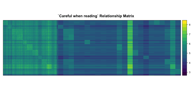
# This matrix now has relationships between all Individuals. Every Bi-parental family is represented by over 50 DH's so if we plot it out, it's kind of hard to see their relationship with the inbred parents which are represented by one genotype each. However you can definitely make out the DH families. I will augment this G-matrix with replicated row entries for the parents so we can visualize this better.
#get names of parents
parents <- rownames(G.matrix)[grep("CFD", rownames(G.matrix), invert = TRUE)]
#replicate every parent 100 times
for(i in 1:length(parents)){
G.matrix <- rbind(G.matrix,
G.matrix[rep(parents[i], 100), 1:ncol(G.matrix)])
}
#Plot fake/augmented G.Matrix
library(lattice)
library(wesanderson)
levelplot(G.matrix[1:nrow(G.matrix),ncol(G.matrix):1],
xlab = NULL, ylab = NULL, scales=list(draw=FALSE),
col.regions = wes_palette("Zissou", 30, type = "continuous"),
main = "`Careful when reading` Relationship Matrix")

#The first third to the left is the DHs followed by the parents. Can you tell which DH came from which parent? Can you tell which one F353 (the central line) is?

#---
#Understanding this matrix
#---

#The genotypes are coded by 0,1,2 by the F353 allele (so homozygous for F353 allele) is 2). This variance terms in this matrix are tracking homozygosity within an inbred or DH. The covariance terms tracking shared alleles between combinations thereof...So why can't we make out the central line if it shares something with all families?...I think because the matrix is adjusted ...by the P vector (see the function)...for the F353 allele which also happens to be the major allele in the overall data. Try commenting out the centering for loop in the function and re-run. See what happens...make sure you "fix" the function back because we need it down-stream. The central line should become clear as in link...
#----
#G-BLUP model
#----

#For the model, we are only interested in the DH families, so lets pull these out of the overall data
prediction.data <- all.data[grep("CFD", all.data$ID),]

#Number of DH lines
nrow(prediction.data)
## [1] 846
#Glance data
prediction.data[1:6,1:6]
##          ID Adjusted.Means abph1.15 abph1.22 ae1.4 ae1.8
## 2 CFD02-003         200.95        2        2     2     2
## 3 CFD02-006         192.01        2        2     2     0
## 4 CFD02-010         207.84        2        2     2     0
## 5 CFD02-024         194.94        2        2     2     0
## 6 CFD02-027         207.84        0        2     2     2
## 7 CFD02-036         195.82        2        2     2     2
#Lets re-create and attach the family information
family.names <- c()
for(i in 1:nrow(prediction.data)){

  f.name <- strsplit(prediction.data$ID[i], split = "-")[[1]][1]
  family.names <- na.omit(c(family.names, f.name))

}

prediction.data <- data.frame(cbind(family=family.names, prediction.data))

#Glance data
prediction.data[1:6,1:6]
##   family        ID Adjusted.Means abph1.15 abph1.22 ae1.4
## 2  CFD02 CFD02-003         200.95        2        2     2
## 3  CFD02 CFD02-006         192.01        2        2     2
## 4  CFD02 CFD02-010         207.84        2        2     2
## 5  CFD02 CFD02-024         194.94        2        2     2
## 6  CFD02 CFD02-027         207.84        0        2     2
## 7  CFD02 CFD02-036         195.82        2        2     2
#----
# G-matrix (DHs only)
#----

#marker matrix
M <- as.matrix(prediction.data[, 4:ncol(prediction.data)])
rownames(M) <- prediction.data$ID

#DH G.Matrix
G.matrix <- make.G.matrix(M)

#Design Matrix for fixed effects
#This matrix assigns every genotype to a family
#Following is one cheap way to make this on R
#Model Phenotype regressed on family without an intercept
model.design <- prediction.data$Adjusted.Means ~ 0 + prediction.data$family
m <- model.frame(model.design, prediction.data)
X <- model.matrix(model.design, m)
rownames(X) <- prediction.data$ID

#Glace design matrix
X[1:6,1:3]
##           prediction.data$familyCFD02 prediction.data$familyCFD03
## CFD02-003                           1                           0
## CFD02-006                           1                           0
## CFD02-010                           1                           0
## CFD02-024                           1                           0
## CFD02-027                           1                           0
## CFD02-036                           1                           0
##           prediction.data$familyCFD04
## CFD02-003                           0
## CFD02-006                           0
## CFD02-010                           0
## CFD02-024                           0
## CFD02-027                           0
## CFD02-036                           0
#What happened here? We fit a model that made such a matrix and then we
#pulled that matrix. Lets fix the column names

#Fix column names
for (i in 1:length(colnames(X))){
  colnames(X)[i] <- strsplit(colnames(X), split = "family")[[i]][2]
}

#Glance design matrix
X[1:2,1:3]
##           CFD02 CFD03 CFD04
## CFD02-003     1     0     0
## CFD02-006     1     0     0
#Model elements
X <- X
G <- G.matrix
y    <- as.vector(prediction.data$Adjusted.Means)

c <- ncol(X) #This is how many families/parents we have
beta <- vector(length = c)

n <- nrow(prediction.data)
I    <- diag(n)
Z    <- diag(n) #Design matrix for random effects

#Equation 1
V = Z %*% G %*% t(Z) + I

#Equation 2
beta_hat = solve(t(X) %*% solve(V) %*% X) %*% t(X) %*% solve(V) %*% y

#Equation 3
u_hat = G %*% t(Z) %*% solve(V) %*% (y - (X %*% beta_hat))
true.bvs <- u_hat

# blup <- X
#
# for(i in 1:ncol(blup)){
#
#   blup[,i] <- blup[,i] * beta_hat[i]
#
# }
#
# blup <- rowSums(blup)
#
# true.blup <- blup + u_hat

#What happened here?
#We used the standard BLUP machinery to estimate breeding values for all individuals using all phenotypic and genotypic records. These estimates will be our "gold-standard". Now, we will hide away parts of the phenotypic records as missing and predict breeding values for these missing ones. Then we will compare these back to our "gold-standard".
#---
# Cross-validation (k-fold)
#---

#Divide data into k sets, train on k-1 sets, predict kth set

k <- 3  #How many folds
CVcycles <- 100 #How many cycles
est.bvs.overall <- c()  #empty object to store results

#----
# G-matrix for total set (same as before)
#----
M <- as.matrix(prediction.data[, 4:ncol(prediction.data)])
rownames(M) <- prediction.data$ID
G.matrix <- make.G.matrix(M)

for (CVcycle in 1:CVcycles) {

#Total set
total.set <- prediction.data
rownames(total.set) <- seq(1, nrow(total.set), 1)

#Set to sample from
sample.set <- rownames(total.set)
estimation.set.size <- round(nrow(prediction.data)/k,0)

#Sample row names (these will be rows we hide phenotypes for)
#i.e. estimation set
estimation.set.index <- sample(sample.set,
                               size = estimation.set.size,
                               replace = FALSE)

#genotypes/lines that make the estimation set
estimation.set <- total.set[estimation.set.index,]$ID

#training set (make estimation set phenotypes "missing")
training.set <-  total.set
training.set$Adjusted.Means[as.numeric(estimation.set.index)] <- NA

#Loop bottleneck (taken out of loop)
# #----
# # G-matrix for total set (same as before)
# #----
# M <- as.matrix(training.set[, 4:ncol(training.set)])
# rownames(M) <- training.set$ID
# G.matrix <- make.G.matrix(M)

#Design matrix for fixed effects...same as before with some modifications
model.design <- training.set$ID ~ 0 + training.set$family
m <- model.frame(model.design, training.set)
X <- model.matrix(model.design, m)
rownames(X) <- training.set$ID

for (i in 1:length(colnames(X))){
  colnames(X)[i] <- strsplit(colnames(X), split = "family")[[i]][2]
}

#We dont know fixed effects for estimation set so set to 0 and remove rows correspoding to the estimation set from design matrix
X[as.character(estimation.set), ] <- 0
X <- X[!rownames(X) %in% estimation.set,]

#Same as before with modifications as in X
Z    <- diag(nrow = nrow(training.set))
colnames(Z) <- rownames(Z)    <- rownames(G.matrix)
Z[as.character(estimation.set), ] <- 0
Z <- Z[!rownames(Z) %in% estimation.set,]

#Same as before with modifications as in X
I    <- diag(nrow = nrow(training.set))
colnames(I) <- rownames(I)    <- rownames(G.matrix)
I <- I[!rownames(I) %in% estimation.set,!colnames(I) %in% estimation.set]

#extract records with all pheno/geno information
training.set.sub <- training.set[!training.set$ID %in% estimation.set, ]

#Model Elements
#same as before with dimensional modifications to adjust for missing-ness
X <- X
G <- G.matrix
I    <- I
Z    <- Z
y    <- as.vector(training.set.sub$Adjusted.Means)
names(y) <- as.character(training.set.sub$ID)
c <- ncol(X) #This is how many families/parents we have
beta <- vector(length = c)
n <- nrow(training.set.sub)

#Equation 1
V = Z %*% G %*% t(Z) + I

#Equation 2
beta_hat = solve(t(X) %*% solve(V) %*% X) %*% t(X) %*% solve(V) %*% y

#Equation 3
u_hat = G %*% t(Z) %*% solve(V) %*% (y - (X %*% beta_hat))

est.bvs <- u_hat

#Combine estimated set with true set
est.bvs <- cbind(est.bvs, true.bvs)

#Extract only the ones that got estimated...drop training set
est.bvs <- est.bvs[estimation.set,]

est.bvs.overall <- rbind(est.bvs.overall, est.bvs)

par(mfrow=c(1,1))
#plot(est.bvs.overall, xlab = "Estimated Breeding Value", ylab = "True Breeding Value")
}

#Plot results (un-comment the plot in line 631 and re-run loop for "magic")
plot(est.bvs.overall, xlab = "Estimated Breeding Value", ylab = "True Breeding Value")

#Accuracy
a <- lm(est.bvs.overall[,1] ~ est.bvs.overall[,2])
paste("accuracy was", round(summary(a)$adj.r.squared,2))
## [1] "accuracy was 0.78"
#---
# Cross-validation (family-fold)
#---

#Divide data by families, train on all families except 1, predict the 1

families <- levels(prediction.data$family) #family names
CVcycles <- 100 #How many cycles
est.bvs.overall <- c()  #empty object to store results

#----
# G-matrix for total set (same as before)
#----
M <- as.matrix(prediction.data[, 4:ncol(prediction.data)])
rownames(M) <- prediction.data$ID
G.matrix <- make.G.matrix(M)

for (CVcycle in 1:CVcycles) {

#Total set
total.set <- prediction.data
rownames(total.set) <- seq(1, nrow(total.set), 1)

#Set to sample from
sample.set <- families

#Sample row names (these will be rows we hide phenotypes for)
#i.e. estimation set
estimation.set.index <- sample(sample.set,
                               size = 1,
                               replace = FALSE)

#genotypes/lines that make the estimation set
estimation.set <- subset(total.set$ID, total.set$family==estimation.set.index)

#training set (make estimation set phenotypes "missing")
training.set <-  total.set
for(i in 1:length(training.set$Adjusted.Means)){

  training.set$Adjusted.Means[i] <-

  ifelse(training.set$family[i] == estimation.set.index, NA,
         training.set$Adjusted.Means[i])

}

#Loop bottleneck (taken out of loop)
# #----
# # G-matrix for total set (same as before)
# #----
# M <- as.matrix(training.set[, 4:ncol(training.set)])
# rownames(M) <- training.set$ID
# G.matrix <- make.G.matrix(M)

#Design matrix for fixed effects...same as before with some modifications
model.design <- training.set$ID ~ 0 + training.set$family
m <- model.frame(model.design, training.set)
X <- model.matrix(model.design, m)
rownames(X) <- training.set$ID

for (i in 1:length(colnames(X))){
  colnames(X)[i] <- strsplit(colnames(X), split = "family")[[i]][2]
}

#We dont know fixed effects for estimation set so set to 0 and remove rows correspoding to the estimation set from design matrix
X[as.character(estimation.set), ] <- 0
X <- X[!rownames(X) %in% estimation.set,]
X <- X[,!colnames(X) %in% estimation.set.index]

#Same as before with modifications as in X
Z    <- diag(nrow = nrow(training.set))
colnames(Z) <- rownames(Z)    <- rownames(G.matrix)
Z[as.character(estimation.set), ] <- 0
Z <- Z[!rownames(Z) %in% estimation.set,]
Z <- Z[,!colnames(Z) %in% estimation.set.index]

#Same as before with modifications as in X
I    <- diag(nrow = nrow(training.set))
colnames(I) <- rownames(I)    <- rownames(G.matrix)
I <- I[!rownames(I) %in% estimation.set,!colnames(I) %in% estimation.set]

#extract records with all pheno/geno information
training.set.sub <- training.set[!training.set$ID %in% estimation.set, ]

#Model Elements
#same as before with dimensional modifications to adjust for missing-ness
X <- X
G <- G.matrix
I    <- I
Z    <- Z
y    <- as.vector(training.set.sub$Adjusted.Means)
names(y) <- as.character(training.set.sub$ID)
c <- ncol(X) #This is how many families/parents we have
beta <- vector(length = c)
n <- nrow(training.set.sub)

#Equation 1
V = Z %*% G %*% t(Z) + I

#Equation 2
beta_hat = solve(t(X) %*% solve(V) %*% X) %*% t(X) %*% solve(V) %*% y

#Equation 3
u_hat = G %*% t(Z) %*% solve(V) %*% (y - (X %*% beta_hat))

est.bvs <- u_hat

#Combine estimated set with true set
est.bvs <- cbind(est.bvs, true.bvs)

#Extract only the ones that got estimated...drop training set
est.bvs <- est.bvs[estimation.set,]

est.bvs.overall <- rbind(est.bvs.overall, est.bvs)

par(mfrow=c(1,1))
#plot(est.bvs.overall, xlab = "Estimated Breeding Value", ylab = "True Breeding Value")
}

#Plot results (un-comment the plot in line 631 and re-run loop for "magic")
plot(est.bvs.overall, xlab = "Estimated Breeding Value", ylab = "True Breeding Value")

#Accuracy
a <- lm(est.bvs.overall[,1] ~ est.bvs.overall[,2])
paste("accuracy was", round(summary(a)$adj.r.squared,2))
## [1] "accuracy was 0.43"